2. Examples

2.1. Heat Capacity

Determine the temperature dependence of the ideal gas heat capacity, \(C_\text{p}^\text{IG}\) for water

>>> import matplotlib.pyplot as plt
>>> from gasthermo.cp import CpIdealGas
>>> I = CpIdealGas(compound_name='Air', T_min_fit=250., T_max_fit=800., poly_order=3)
>>> I.eval(300.), I.Cp_units
(29.00369515161452, 'J/mol/K')
>>> I.eval(300.)/I.MW
1.0015088104839267
>>> # we can then plot and visualize the resutls
>>> fig, ax = I.plot()
>>> fig.savefig('docs/source/air.png')
>>> del I

And we will get something that looks like the following

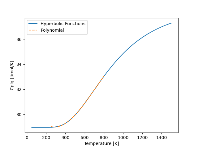
and we notice that the polynomial (orange dashed lines) fits the hyperbolic function well.

2.2. Equations of State

2.2.1. Cubic

>>> from gasthermo.eos.cubic import PengRobinson, RedlichKwong, SoaveRedlichKwong
>>> P = 8e5  # Pa
>>> T = 300. # K
>>> PengRobinson(compound_name='Propane').iterate_to_solve_Z(P=P, T=T)
0.8568255826283575
>>> RedlichKwong(compound_name='Propane').iterate_to_solve_Z(P=P, T=T)
0.8712488647564147
>>> cls_srk = SoaveRedlichKwong(compound_name='Propane')
>>> Z = cls_srk.iterate_to_solve_Z(P=P, T=T)
>>> Z
0.8652883337846884
>>> # calculate residual properties
>>> from chem_util.chem_constants import gas_constant as R
>>> V = Z*R*T/P
>>> cls_srk.S_R_R_expr(P, V, T)
-0.3002887932902908
>>> cls_srk.H_R_RT_expr(P, V, T)
-0.4271408507179967
>>> cls_srk.G_R_RT_expr(P, V, T) - cls_srk.H_R_RT_expr(P, V, T) + cls_srk.S_R_R_expr(P, V, T)
0.0

2.2.2. Virial

>>> from gasthermo.eos.virial import SecondVirial
>>> Iv2 = SecondVirial(compound_name='Propane')
>>> Iv2.calc_Z_from_units(P=8e5, T=300.)
0.8726051032825523

2.3. Mixtures

Note

currently only implemented for virial equation of state

2.3.1. Residual Properties

Below, an example is shown for calculating residual properties of THF/Water mixtures

>>> from gasthermo.eos.virial import SecondVirialMixture
>>> P, T = 1e5, 300.
>>> mixture = SecondVirialMixture(compound_names=['Water', 'Tetrahydrofuran'], k_ij=0.)
>>> import matplotlib.pyplot as plt
>>> fig, ax = mixture.plot_residual_HSG(P, T)
>>> fig.savefig('docs/source/THF-WATER.png')

So that the results look like the following

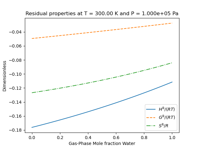
We note that the residual properties will not always vanish in the limit of pure components like excess properties since the pure-components may not be perfect gases.

2.4. Other Utilities

Determine whether a single real root of the cubic equation of state can be used for simple computational implementation. In some regimes, the cubic equation of state only has 1 real root–in this case, the compressibility factor can be obtained easily.

>>> from gasthermo.eos.cubic import PengRobinson
>>> pr = PengRobinson(compound_name='Propane')
>>> pr.num_roots(300., 5e5)
3
>>> pr.num_roots(100., 5e5)
1

2.5. Gotchas

• All units are SI units