1. Getting Started
1.2. Single-Component Examples
1.2.1. Heat Capacity
Determine the temperature dependence of the ideal gas heat capacity, \(C_\text{p}^\text{IG}\) for water
>>> import matplotlib.pyplot as plt
>>> from gasthermo.cp import CpIdealGas
>>> I = CpIdealGas(compound_name='Air', T_min_fit=250., T_max_fit=800., poly_order=3)
>>> I.eval(300.), I.Cp_units
(29.00369, 'J/mol/K')
>>> I.eval(300.)/I.MW
1.001508
>>> # we can then plot and visualize the resutls
>>> fig, ax = I.plot()
>>> fig.savefig('docs/source/air.png')
>>> del I
And we will get something that looks like the following
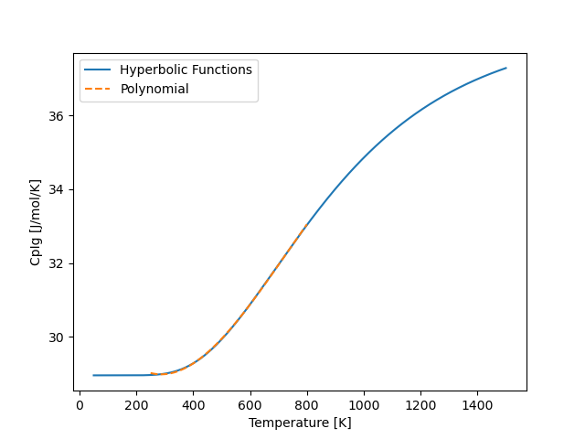
and we notice that the polynomial (orange dashed lines) fits the hyperbolic function well.
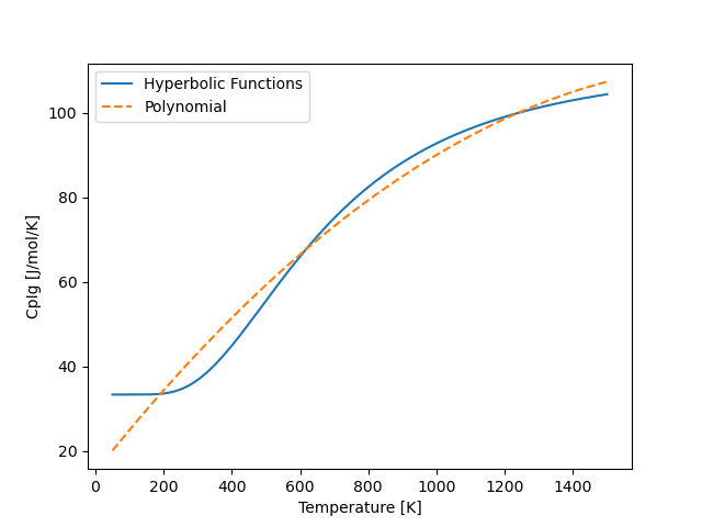
Automatically tries to raise errors if fit is not good enough:
>>> from gasthermo.cp import CpIdealGas
>>> I = CpIdealGas(compound_name='Methane')
Traceback (most recent call last):
    ...
Exception: Fit is too poor (not in (0.99,1)) too large!
Try using a smaller temperature range for fitting
and/or increasing the number of fitting points and polynomial degree.
See error path in error-*dir
This will lead to an error directory with a figure saved in it that looks like the following:
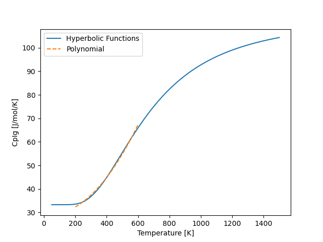
Usually, we wont need an accurate function over this entire temperature range. Lets imagine that we are interested instead in a temperature interval between 200 and 600 K. In this case
>>> I = CpIdealGas(compound_name='Methane', T_min_fit=200., T_max_fit=600.)
And then we can save the results to a file
>>> fig = plt.figure()
>>> fig, ax = I.plot(fig=fig)
>>> fig.savefig('docs/source/cp-methane-fixed.png')
Which leads to a much better fit, as shown below
1.2.2. Cubic Equations of State
>>> from gasthermo.eos.cubic import PengRobinson, RedlichKwong, SoaveRedlichKwong
>>> P = 8e5  # Pa
>>> T = 300. # K
>>> PengRobinson(compound_name='Propane').iterate_to_solve_Z(P=P, T=T)
0.85682
>>> RedlichKwong(compound_name='Propane').iterate_to_solve_Z(P=P, T=T)
0.87124
>>> cls_srk = SoaveRedlichKwong(compound_name='Propane')
>>> Z = cls_srk.iterate_to_solve_Z(P=P, T=T)
>>> Z
0.86528
>>> # calculate residual properties
>>> from chem_util.chem_constants import gas_constant as R
>>> V = Z*R*T/P
>>> cls_srk.S_R_R_expr(P, V, T)
-0.30028
>>> cls_srk.H_R_RT_expr(P, V, T)
-0.42714
>>> cls_srk.G_R_RT_expr(P, V, T) - cls_srk.H_R_RT_expr(P, V, T) + cls_srk.S_R_R_expr(P, V, T)
0.0
1.2.3. Virial Equation of State
>>> from gasthermo.eos.virial import SecondVirial
>>> Iv2 = SecondVirial(compound_name='Propane')
>>> Iv2.calc_Z_from_units(P=8e5, T=300.)
0.87260
1.2.4. Other Utilities
Determine whether a single real root of the cubic equation of state can be used for simple computational implementation. In some regimes, the cubic equation of state only has 1 real root–in this case, the compressibility factor can be obtained easily.
>>> from gasthermo.eos.cubic import PengRobinson
>>> pr = PengRobinson(compound_name='Propane')
>>> pr.num_roots(300., 5e5)
3
>>> pr.num_roots(100., 5e5)
1
Input custom thermodynamic critical properties
>>> from gasthermo.eos.cubic import PengRobinson
>>> dippr = PengRobinson(compound_name='Methane')
>>> custom = PengRobinson(compound_name='Methane', cas_number='72-28-8',
...                       T_c=191.4, V_c=0.0001, Z_c=0.286, w=0.0115, MW=16.042, P_c=0.286*8.314*191.4/0.0001)
>>> dippr.iterate_to_solve_Z(T=300., P=8e5)
0.9828233
>>> custom.iterate_to_solve_Z(T=300., P=8e5)
0.9823877
If we accidentally input the wrong custom units,
it is likely that gasthermo.critical_constants.CriticalConstants will catch it.
>>> from gasthermo.eos.cubic import PengRobinson
>>> PengRobinson(compound_name='Methane', cas_number='72-28-8',
...                       T_c=273.-191.4, V_c=0.0001, Z_c=0.286, w=0.0115, MW=16.042, P_c=0.286*8.314*191.4/0.0001)
Traceback (most recent call last):
...
AssertionError: Percent difference too high for T_c
>>> PengRobinson(compound_name='Methane', cas_number='72-28-8',
...                       T_c=191.4, V_c=0.0001*100., Z_c=0.286, w=0.0115, MW=16.042, P_c=0.286*8.314*191.4/0.0001)
Traceback (most recent call last):
...
AssertionError: Percent difference too high for V_c
>>> PengRobinson(compound_name='Methane', cas_number='72-28-8',
...                       T_c=191.4, V_c=0.0001, Z_c=2.86, w=0.0115, MW=16.042, P_c=0.286*8.314*191.4/0.0001)
Traceback (most recent call last):
...
AssertionError: Percent difference too high for Z_c
>>> PengRobinson(compound_name='Methane', cas_number='72-28-8',
...                       T_c=191.4, V_c=0.0001, Z_c=0.286, w=1.115, MW=16.042, P_c=0.286*8.314*191.4/0.0001)
Traceback (most recent call last):
...
AssertionError: Percent difference too high for w
>>> PengRobinson(compound_name='Methane', cas_number='72-28-8',
...                       T_c=191.4, V_c=0.0001, Z_c=0.286, w=0.0115, MW=18.042, P_c=0.286*8.314*191.4/0.0001)
Traceback (most recent call last):
...
AssertionError: Percent difference too high for MW
>>> PengRobinson(compound_name='Methane', cas_number='72-28-8',
...                       T_c=191.4, V_c=0.0001, Z_c=0.286, w=0.0115, MW=18.042, P_c=0.286*0.008314*191.4/0.0001)
Traceback (most recent call last):
...
AssertionError: Percent difference too high for P_c
It performs the checks by comparing to the DIPPR [RWO+07] database and asserting that the values are within a reasonable tolerance
1.3. Mixture Examples
Note
For non-ideal gases, currently only implemented for virial equation of state
1.3.1. Residual Properties
Below, an example is shown for calculating residual properties of THF/Water mixtures
>>> from gasthermo.eos.virial import SecondVirialMixture
>>> P, T = 1e5, 300.
>>> mixture = SecondVirialMixture(compound_names=['Water', 'Tetrahydrofuran'], k_ij=0.)
>>> import matplotlib.pyplot as plt
>>> fig, ax = mixture.plot_residual_HSG(P, T)
>>> fig.savefig('docs/source/THF-WATER.png')
So that the results look like the following
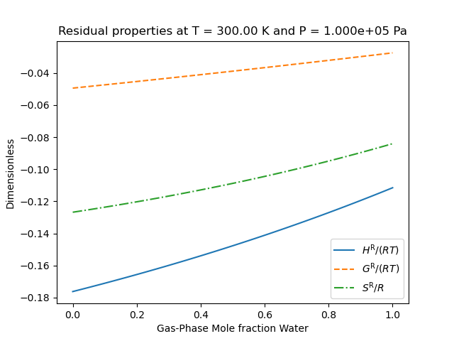
We note that the residual properties will not always vanish in the limit of pure components like excess properties since the pure-components may not be perfect gases.
1.3.2. Partial Molar Properties
>>> from gasthermo.partial_molar_properties import Mixture
>>> cp_kwargs = dict(T_min_fit=200., T_max_fit=600.)
>>> I = Mixture(
...     [dict(compound_name='Methane', **cp_kwargs), dict(compound_name='Ethane', **cp_kwargs)],
...      compound_names=['Methane', 'Ethane'],
...      ideal=False,
...     )
>>> I.T_cs
[190.564, 305.32]
>>> I.cas_numbers
['74-82-8', '74-84-0']
The reference state is the pure component at \(P=0\) and \(T=T_\text{ref}\). The reference temperature is \(T_\text{ref}\) and defaults to 0 K. But different values can be used, as shown below
>>> I.enthalpy(ys=[0.5, 0.5], P=1e5, T=300.)
9037.3883
>>> I.enthalpy(ys=[0.5, 0.5], P=1e5, T=300., T_ref=0.)
9037.3883
>>> I.enthalpy(ys=[0.5, 0.5], P=1e5, T=300., T_ref=300.)
-31.33905
>>> I.ideal = True
>>> I.enthalpy(ys=[0.5, 0.5], P=1e5, T=300., T_ref=300.)
0.0
And we observe that the enthalpy can be non-zero for real gases when the reference temperature is chosen to be the same as the temperature of interest, since the enthalpy departure function is non-zero.
However, for a real gas,
>>> I.ideal = False
in the limit that the gas has low pressure and high temperature,
>>> I.enthalpy(ys=[0.5, 0.5], P=1., T=500., T_ref=500.)
-0.000111958
In the limit that the gas becomes a pure mixture, we recover the limit that \(\bar{H}_i^\text{pure}=H^\text{pure}\) or \(\bar{H}_i^\text{pure}-H^\text{pure}=0.\)
>>> kwargs = dict(ys=[1., 0.], P=1e5, T=300.)
>>> I.enthalpy(**kwargs)-I.bar_Hi(I.cas_numbers[0], **kwargs)
0.0
>>> kwargs = dict(ys=[0., 1.], P=1e5, T=300.)
>>> I.enthalpy(**kwargs)-I.bar_Hi(I.cas_numbers[1], **kwargs)
0.0
Using the second order virial equation of state we can perform these same calculations on multicomponent mixtures, as shown below
Note
all units are SI units, so the enthalpy here is in J/mol
>>> cp_kwargs = dict(T_min_fit=200., T_max_fit=600.)
>>> M = Mixture(
...     [dict(compound_name='Methane', **cp_kwargs),
...      dict(compound_name='Ethane', **cp_kwargs), dict(compound_name='Ethylene', **cp_kwargs),
...      dict(compound_name='Carbon dioxide', **cp_kwargs)],
...      compound_names=['Methane', 'Ethane', 'Ethylene', 'Carbon dioxide'],
...      ideal=False,
...     )
>>> M.enthalpy(ys=[0.1, 0.2, 0.5, 0.2], P=10e5, T=300.)
7432.66593
>>> M.enthalpy(ys=[1.0, 0.0, 0.0, 0.0], P=10e5, T=300.) - M.bar_Hi(M.cas_numbers[0], ys=[1.0, 0.0, 0.0, 0.0], P=10e5, T=300.)
0.0
Another simple check is to ensure that we get the same answer regardless of the order of the compounds
>>> N = Mixture(
...     [dict(compound_name='Ethane', **cp_kwargs),
...      dict(compound_name='Methane', **cp_kwargs), dict(compound_name='Ethylene', **cp_kwargs),
...      dict(compound_name='Carbon dioxide', **cp_kwargs)],
...      compound_names=['Ethane', 'Methane', 'Ethylene', 'Carbon dioxide'],
...      ideal=False,
...     )
>>> M.enthalpy(ys=[0.4, 0.3, 0.17, 0.13], P=5e5, T=300.) - N.enthalpy(ys=[0.3, 0.4, 0.17, 0.13], P=5e5, T=300.)
0.0
And that, further, a mixture with an extra component that is not present (mole fraction 0.) converges to an \(N-1\) mixture
>>> Nm1 = Mixture(  # take out CO2
...     [dict(compound_name='Ethane', **cp_kwargs),
...      dict(compound_name='Methane', **cp_kwargs), dict(compound_name='Ethylene', **cp_kwargs)],
...      compound_names=['Ethane', 'Methane', 'Ethylene'],
...      ideal=False,
...     )
>>> N.enthalpy(ys=[0.4, 0.3, 0.3, 0.], P=5e5, T=300.) - Nm1.enthalpy(ys=[0.4, 0.3, 0.3], P=5e5, T=300.)
0.0
1.4. Gotchas
All units are SI units